A sales capacity model is a disciplined way to answer one finance question: how many fully productive sellers do we need, when do we need them, and what revenue should that capacity produce?
In our blog, we leveraged our AI revenue strategist Atlas to weave in an example through our 10-step sales capacity model guide. Assuming a SaaS new-logo motion, here’s the order to build it in against a concrete example: an illustrative $10M new ARR plan across SMB, Mid-Market, and Enterprise.
Step 1: Start With the Revenue Target
Define the number the sales team is responsible for:
- New ARR
- Expansion ARR
- Renewal base, if renewals sit in the same team
Keep these separate. A capacity model gets distorted fast if new business and retention revenue are blended.
For our example, the target is simple: $10M in new ARR for the fiscal year. Everything below builds toward whether the team, as staffed, can actually produce that number.
Step 2: Segment the GTM Motion
Build separate lanes for each materially different motion:
- SMB
- Mid-market
- Enterprise
- Channel/partner
- CS/AM expansion
Each lane should have its own OTE, quota, ramp time, win rate, sales cycle, and expected deal size. A mid-market AE and an enterprise AE should almost never share one capacity assumption set.
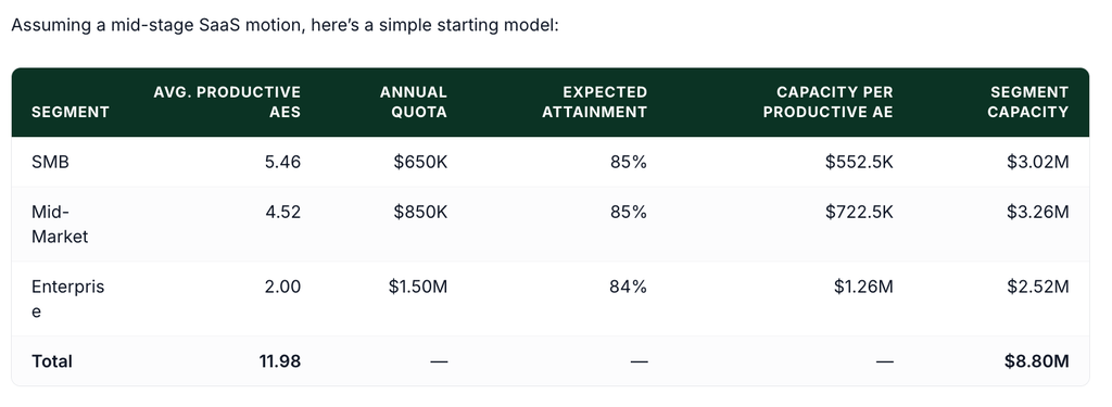
Our $10M plan runs across three lanes: SMB, Mid-Market, and Enterprise. Here’s how the capacity breaks down once each segment’s assumptions are applied (the math for each column is explained in the next two steps):
| Segment | Avg. productive AEs | Annual quota | Expected attainment | Capacity per productive AE | Segment capacity |
|---|---|---|---|---|---|
| SMB | 5.46 | $650K | 85% | $552.5K | $3.02M |
| Mid-Market | 4.52 | $850K | 85% | $722.5K | $3.26M |
| Enterprise | 2.00 | $1.50M | 84% | $1.26M | $2.52M |
| Total | 11.98 | n/a | n/a | n/a | $8.80M |
Step 3: Define Productive Capacity Per Fully Ramped Rep
This is the core output of the model. Most CFO teams use one of two methods.
Quota-based: fully ramped rep capacity = annual quota × expected attainment.
Example: quota of $800K ARR at 80% expected attainment produces $640K ARR of productive capacity per rep.
Funnel-based: capacity = opportunities × win rate × ACV.
Example: 40 qualified opps a year, a 25% win rate, and a $70K ACV produce $700K ARR of capacity.
If the quota-based and funnel-based views don’t roughly reconcile, the quota is likely aspirational rather than capacity-backed.
Applying the quota-based method to each of our three segments:
- SMB: $650K quota × 85% attainment = $552.5K capacity per AE
- Mid-Market: $850K quota × 85% attainment = $722.5K capacity per AE
- Enterprise: $1.50M quota × 84% attainment = $1.26M capacity per AE
Those per-AE figures are what get multiplied by ramp-adjusted headcount in the next step to produce the segment capacity numbers shown in the table above.
Step 4: Apply Ramping by Cohort and Hire Date
Do not count every head as a full-year producer. For each hire cohort, estimate months to productivity, percent productivity by month or quarter, and time in seat during the fiscal year.
A simple ramp curve:
- Q1 in role: 25%
- Q2: 50%
- Q3: 75%
- Q4 and beyond: 100%
So a rep hired July 1 is not one head; they may only contribute 40 to 50% of annualized capacity in that fiscal year.
This is exactly why our example shows 11.98 average productive AEs across the three segments rather than a round headcount number. That 11.98 is ramp-adjusted selling capacity, not payroll headcount. A Q2 hire might contribute only 0.5 to 0.7 productive AE-years depending on when in the quarter they start and how fast they ramp.
Step 5: Adjust for Attrition and Vacancies
This is where most models become too optimistic. Include voluntary and involuntary attrition, time to backfill, manager span constraints, and recruiting lead time.
A practical finance adjustment: net productive reps = gross productive reps (ending headcount) minus vacancy drag and ramp drag. If you skip vacancy time, you will usually overstate output by double digits.
Back in our example, an open backfill sitting vacant for two months might reduce capacity by 0.15 to 0.20 AE-years on its own. Stack a few of those vacancy gaps on top of normal ramp drag, and 14 people on payroll can easily translate into something closer to 12 productive AE-years, well below what the raw headcount number would suggest.
Step 6: Convert Headcount Into Capacity
At this point, the math becomes straightforward:
Net revenue capacity = sum of each cohort’s ramp-adjusted productive capacity
Simple structure: beginning fully ramped reps, plus new hires (ramp-adjusted), minus attrition (time-adjusted), equals average productive reps. Average productive reps × productive capacity per rep = revenue capacity. This is the number to compare against the plan.
Rolling up our three segments: SMB at $3.02M, Mid-Market at $3.26M, and Enterprise at $2.52M totals $8.80M of modeled capacity.
Against the $10.0M target, that leaves a gap of:
$10.0M − $8.80M = $1.20M
So the model, as staffed, is about 12% short before pipeline risk, slippage, or execution variance even enters the picture.
To close that $1.20M gap, you roughly need one of the following:
- About 1 additional fully productive Enterprise AE equivalent ($1.20M ÷ $1.26M ≈ 0.95)
- About 1.7 additional fully productive Mid-Market AE equivalents ($1.20M ÷ $722.5K ≈ 1.66)
- About 2.2 additional fully productive SMB AE equivalents ($1.20M ÷ $552.5K ≈ 2.17)
Put differently, the system needs about 1.6 more productive AE-years somewhere, whether that comes from one segment or is spread across a few.
Step 7: Check Whether Pipeline Coverage Supports the Model
Capacity alone does not create revenue. Stress test it: required pipeline = bookings target ÷ win rate; required SQOs per rep = quota ÷ ACV ÷ win rate. Then check whether marketing and SDR creation can actually feed that load.
If the model says 20 AEs can produce the plan, but pipeline generation only supports 14, the capacity model is economically incomplete.
Running that check on our example segments:
- SMB: $650K quota ÷ $20K ACV ÷ 25% win rate = 130 opps/year per AE
- Mid-Market: $850K quota ÷ $50K ACV ÷ 22% win rate = 77 opps/year per AE
- Enterprise: $1.50M quota ÷ $150K ACV ÷ 18% win rate = 56 opps/year per AE
If marketing and SDR capacity can’t support that volume across all three segments, the $8.80M capacity figure is overstated, even if the headcount looks right on paper. The hiring gap from Step 6 and a pipeline gap here can both be true at once, and both need to be closed.
Step 8: Tie It to Cost
Now connect revenue capacity to sales cost: fully loaded rep cost, manager cost, SDR support, sales engineering/support ratios, and commissions at target and at expected attainment.
This gives you cost per productive rep, sales cost as a percent of ARR/bookings, and payback expectations. That is usually the CFO’s view that matters most, and it’s worth running for each of the three segments separately, since loaded cost and commission structures typically differ by motion.
Step 9: Run Three Cases, Not One
Use at least a base case (expected attainment, expected hiring pace), an upside case (stronger ramp, lower attrition), and a downside case (slower hiring, weaker productivity, higher attrition). A capacity model should show sensitivity, not false precision.
Applied to the example: the $8.80M base case already sits $1.2M under plan. It’s worth running that same model with a faster Enterprise ramp and lower Mid-Market attrition to see how much of the gap upside conditions could close on their own, versus how much has to come from added headcount or pipeline.
Step 10: Pressure-Test With Reality
Before using the model for planning, compare it against the last four quarters of actual attainment, actual ramp curves, actual attrition, and actual ACV and win rate by segment. If history says reps ramp in seven months, a four-month model is not a plan; it’s a hope.
If, say, Enterprise reps have historically taken nine months to ramp rather than the four quarters assumed in Step 4, the true capacity number is lower than $8.80M, and the gap to plan is larger than $1.2M. This step is what keeps the rest of the model honest.
The Simplest Formula Set
If you want a clean first-pass model, use:
- Productive capacity per fully ramped AE = quota × expected attainment
- Average productive AEs = starting productive AEs + ramp-adjusted hires − attrition/vacancy drag
- Revenue capacity = average productive AEs × productive capacity per AE
- Gap to plan = revenue target − revenue capacity
What Usually Goes Wrong
- Using quota instead of actual expected productivity
- Counting new hires as full-year contributors
- Ignoring attrition and time-to-backfill
- Not separating segments/motions
- Forgetting pipeline creation limits
Design, track, and manage variable incentives with QuotaPath. Give your RevOps, finance, and sales teams transparency into sales compensation.
Talk to SalesThe Key Takeaway
Our capacity plan should be built on ramp-adjusted productive sellers, not end-of-quarter headcount, because hiring pace and vacancy drag usually matter as much as quota setting.
On a $10M new ARR plan, the relevant number is ramp-adjusted productive capacity, not ending headcount. Based on the assumptions above, the team is carrying about $8.8M in modeled capacity, leaving a $1.2M gap to plan for before factoring in pipeline coverage.
For additional help in building out your go-to-market strategy, check out Atlas for free.